Neural Networks Backpropagation

Gradient

Video

The gradient captures all the partial derivative information of a scalar-valued multivariable function. Created by Grant Sanderson.

A vector of partial derivatives for a multivariate function.

Gives the direction of steepest ascent (descent) of the function.

The directional derivative

The directional derivative is the dot product between the gradient and the unit vector in that direction.

In our case we have the C as the cost function, and the partial derivatives for the weights and biases. We want to descent the gradient of the cost function.

The dimensionality of the gradient space is given by the number of weights and biases for the model.

The chain rule

The chain rule tells us that the derivative of a composite function is equal to the product of the derivatives of each of its parts.

df(g(x))/dx = df/dg * dg/dx

We have a cost function L, and we want to find the partial derivative of L with respect to each parameter. We can do that by using the chain rule:

if L = fg, and f=h+k => dL/df = g, dL/dg = f, df/dh = 1, df/dk = 1. Using the chain rule, dL/dh = dL/dfdf/dh and so on. dL/dh is the gradient of h; how much does h impact the gradient descent.

Remarks:

• a plus sign distributes the gradient of a parent to its children.
• we can only influence leaf nodes during gradinet descent. In the example above, we can only influence h,k and g
• because a parameter can be referenced more than once, the gradients have to be summed up instead of overwritted at parameter level.

Neuron

We have n inputs, x-es each with a weight, w-s. And a bias b. Then we have an activation function f, a squashing function. The value of the neuron is f(sum(xi*wi) + b).

Layer

A set of n neurons

MLP: multi-layer perceptron

A chaining of multiple layers: An input layer, 0 to multiple hidden layers and the output layer. Each neuron in Layer n is connected to each neuron in Layer n-1.

A forward pass: we take a set of input values and forward pass through the entire network. There’s an activation function at the end with the main goal of squashing the values. Why do we need squashing: to make sure that the output is bounded between 0 and 1. We call the output of this layer the activations. Multiple samples are processed in parallel in a batch and a loss or cost function is computed over the predictions of each sample versus the extected values.

Backward propagation is called on the loss function to calculate the gradients for each parameter over the entire batch. Based on the gradients, we update the parameters in the direction that reduces the loss (the gradient descent).

How to choose a proper learning rate?

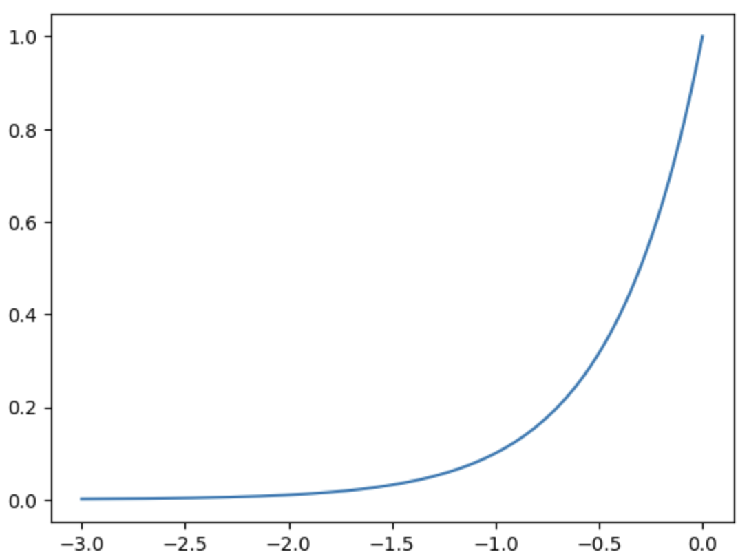
Instead of a static learning rate, build a dynamic learning rate with the powers of 10 between -3 and 0; 1000 of them

lre = torch.linspace(-3, 0, 1000)
lrs = 10**lre

This will be between 0.001 and 1, but exponentiated.

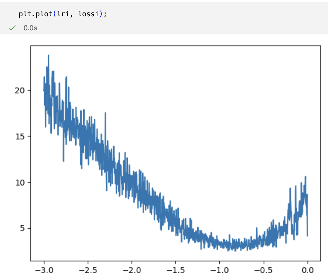
Run a training loop with the dynamic learning rate, save the loss and plot it. You get something like this: So the best rate is between the -1 and -0.5 exponent of 10.

How to arrange the data

Have 3 splits for the dataset:

• Training set (80%) - used to optimize the parameters
• Validation set (10%) - used for development of the hiperparameters (size of the emb, batch etc)
• Test set (10%) - used at the end to test the final model.

Logits

The logits are the raw output of the neural network before passing them through an activation function.

Activation functions

An activation function is used to introduce non-linearity in the model, and it’s usually applied at the end of the linear part of the network. Examples of activation functions are: ReLU, LeakyReLU, ELU, SELU, Sigmoid, Tanh and many more.

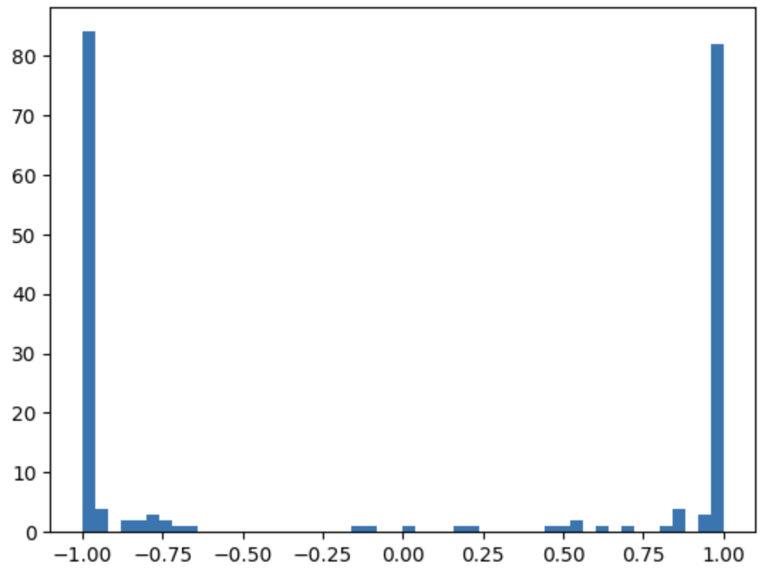
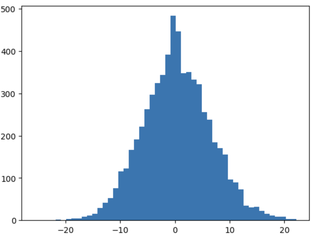
The distribution for a not-normalized activation function for 32 samples on 200 newurons This is triggered by the preactivations that are widely distributed. Whatever is lower than -1 is squashed into -1 and whatever is higher than +1 is squashed into +1.

The problem is that during differentiatiation, in 1 and -1, it goes to 0 and makes the network untrainable, that newuron will not learn anything. It’s called a dead neuron.

How to solve it: normalize at initialization the parameters that contribute to the preactivations:

W1 = torch.randn((block_size * n_embed, n_hidden), generator=g) * 0.2
b1 = torch.randn(n_hidden, generator=g) * 0.01

Softmax

The softmax is a normalizing function that converts the logits into probabilities. At the beginning the softmax can be confidently wrong. That’s because the parameters are not normalized and the preactivations are widely distributed.

How to solve it: normalize at initialization the parameters that contribute to the logits, hence softmax:

W2 = torch.randn((n_hidden, vocab_size), generator=g) * 0.01
b2 = torch.randn(vocab_size, generator=g) * 0

Normalization

How to get rid of the magic numbers used in the previous examples? What we want is a unit gaussian data distribution. That means, a standard deviation of one.

Divide the parameters by the square root of the fan-in. The fan-in is the number of inputs that a neuron receives. Multiple it with a gain, that in case of tanh is 5/3. See torch.nn.init

Batch normalization

Normalize the preactivation to be unit gaussian. The mean and standard deviation are computed over the batch dimension.

    hpreact = bngain * ((hpreact - hpreact.mean(0, keepdim=True))/hpreact.std(0, keepdim=True)) + bnbias

bngain and bnbias are learnable parameters introduced in order to allow the training to go outside of the unit gaussian.